When the Springs Stop Being Simple - Nonlinearity and Chaos

Everything in the last four posts has rested on a single assumption, stated quietly but used constantly: the oscillations are small. Small enough that restoring forces are proportional to displacement. Small enough that the wave equation stays linear, that superposition holds, that the dispersion relation describes behaviour across all amplitudes equally. The band gaps we derived in Post 4 are real, they work in experiments, and they are beautiful. But they belong to a world where amplitude doesn’t matter.

Push the system hard enough, and that world ends.

This is the post where we leave the clean linear regime and enter territory that is messier, richer, and considerably closer to the questions I actually care about. Nonlinearity is not a failure of metamaterial design; it is, if you approach it deliberately, a feature. And chaos, which sits at the far end of the nonlinear spectrum, turns out to be a surprisingly effective tool for sound attenuation. Let me explain why.

Why We Assumed Small Oscillations

#

The linear approximation isn’t lazy physics. It’s the first term of a Taylor expansion, and most of the time it’s all you need.

For any smooth restoring force F(x), we can expand around the equilibrium position x = 0:

$$F(x) = F(0) + F’(0),x + \frac{1}{2}F’’(0),x^2 + \frac{1}{6}F’’’(0),x^3 + \ldots$$

At equilibrium, F(0) = 0. For a symmetric potential (the standard assumption), the even terms vanish too. What remains, for small x, is simply F ≈ F’(0) x = −kx: a spring force proportional to displacement. This is Hooke’s law. It’s not a physical fact about springs; it’s a mathematical fact about smooth functions near their minima. Every spring obeys it at small enough amplitudes.

The catch is that word “enough.” As displacement grows, the higher-order terms become significant. The spring stops being simple. And the consequences ripple through every analysis that assumed it was.

The Duffing Oscillator: When the Cubic Term Matters

#

Add the leading nonlinear correction to the restoring force:

$$F = -kx - \alpha x^3$$

This is the Duffing oscillator, first studied systematically by Georg Duffing in 1918. The coefficient α controls the character of the nonlinearity. When α > 0, the spring stiffens as displacement grows: the effective spring constant increases with amplitude, and the oscillator’s natural frequency rises. When α < 0, the spring softens, frequency falls. Both cases occur in real physical systems depending on the material and geometry involved.

The frequency-response curve that results from this single extra term is already qualitatively different from anything a linear oscillator produces. In a linear system, the resonance peak is symmetric: the oscillator responds most strongly at exactly the natural frequency, and the response falls off on both sides. In the Duffing oscillator, the peak leans. The hardening case (α > 0) bends the resonance curve to the right; the softening case bends it left. At high enough drive amplitudes, the curve folds back on itself, creating a region where three different steady-state responses are possible at the same driving frequency. Two are stable; one is not. Which stable state the system finds depends on its history, specifically on whether the driving frequency is being swept upward or downward. This hysteresis, a property linear systems fundamentally cannot exhibit, is the first sign that amplitude is starting to matter.

In the context of a metamaterial resonator, this matters because the resonant frequency of each internal oscillator is no longer a fixed number. It depends on how hard you’re driving it. And when the resonant frequency shifts, the band gap shifts with it.

Amplitude-Dependent Band Gaps

#

This is where the physics of acoustic metamaterials becomes genuinely interesting. In the linear theory, a band gap sits at a fixed position in frequency space, set by the resonator mass and stiffness. You design for a target frequency, the gap appears there, and it stays there regardless of signal amplitude. Elegant, but also fragile: a narrowband attenuator that may perform well in laboratory conditions and struggle when exposed to high-amplitude real-world sources.

Nonlinear resonators change this picture. When the resonators are Duffing-type (as in a metamaterial with stiff, geometrically nonlinear spring elements), the band gap position shifts with amplitude. A hardening resonator pushes the gap to higher frequencies as amplitude grows; a softening one moves it lower. This is not a defect. Designed carefully, it means the metamaterial can maintain suppression across a broader range of conditions than a linear device ever could, because the gap tracks the incoming energy level rather than remaining fixed.

Fang, Wen, Bonello, Yin, and Yu demonstrated this in 2017 in a landmark Nature Communications paper that sits close to the centre of everything I’m working on. Their nonlinear acoustic metamaterials, built around Duffing oscillator resonators, showed ultra-low frequency band gaps, below 100 Hz, achieved through purely nonlinear mechanisms rather than large mass or geometric scale. Critically, increasing the drive amplitude didn’t destroy the band gap: it widened it. The gap expanded adaptively with the incoming intensity, and at sufficiently high amplitudes the attenuation became broadband, covering frequency ranges that no single linear resonator could span. They extended this analysis in a companion paper in New Journal of Physics the same year, working through the wave propagation theory for a one-dimensional nonlinear metamaterial lattice and showing that strong nonlinearity fundamentally changes the character of wave suppression compared to linear Bragg scattering or local resonance. Bae and Oh (2020), in the Journal of the Mechanics and Physics of Solids, formalised this as the concept of an “amplitude-induced bandgap”: a class of suppression zone that exists only in nonlinear systems and has no linear analogue.

The design implication is significant. If you need to suppress low-frequency sound at varying amplitude levels, a linear metamaterial requires either a wide static gap (which means heavy, softly coupled resonators and attendant engineering constraints) or active tuning (which means sensors, actuators, and feedback control). A nonlinear metamaterial tuned to the right operating regime gives you adaptive bandwidth for free, as a passive consequence of the physics.

Bifurcations: The Route to Chaos

#

Amplitude-dependent band gaps are already useful. But they’re just the beginning of what happens as drive amplitude increases further. The system starts to undergo bifurcations.

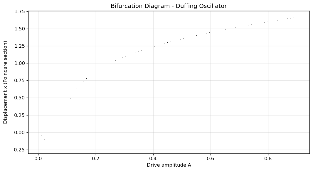
A bifurcation is a qualitative change in the long-run behaviour of a dynamical system as a parameter crosses a critical threshold. The simplest and most important for our purposes is the period-doubling bifurcation. Below the threshold, a Duffing oscillator driven at frequency f settles into a periodic orbit with the same period as the drive. Cross the threshold, and the response period doubles: the oscillator now takes two drive cycles to return to the same state. Cross another threshold, and the period doubles again. Then again.

This cascade of period doublings, if you plot the long-run amplitude of the response against the drive amplitude on a bifurcation diagram, produces one of the most recognisable structures in nonlinear dynamics: the Feigenbaum tree. A single branch at low amplitude, splitting at the first bifurcation, splitting again, splitting again, and then, above a critical amplitude, the branches become dense and overlap. The system’s response no longer repeats at any fixed period. It has entered chaos.

Chaos here has a precise mathematical meaning, not the colloquial one. A chaotic dynamical system is deterministic: given exact initial conditions, the trajectory is determined. But it is sensitively dependent on those conditions. Two trajectories that start arbitrarily close together diverge exponentially in time. No finite measurement precision can predict long-run behaviour. This sensitivity is quantified by the Lyapunov exponent: the average rate of exponential separation between nearby trajectories in phase space. A positive Lyapunov exponent is the signature of chaos. A negative one indicates stable periodic behaviour. The transition from negative to positive, as drive amplitude increases through the bifurcation cascade, is the transition from order to chaos.

What Chaos Does to Sound Attenuation

#

Here is where the argument becomes genuinely exciting, and where it connects directly to my own research angle.

In a chaotic metamaterial resonator, energy injected at one frequency spreads across a broad spectral range. The coupling between the drive frequency and the higher harmonics and subharmonics is strong, nonlinear, and amplitude-dependent. The resonator does not oscillate cleanly at one frequency and radiate at one frequency; it produces a rich, broadband response. From the perspective of wave transmission through the metamaterial, this is attenuation: energy that enters the chain as a coherent wave at a specific frequency does not exit as a coherent wave at that frequency. It has been scattered, mode-mixed, and spread.

Fang and colleagues, in their 2020 Physical Review B paper, distinguished carefully between two overlapping nonlinear mechanisms: the adaptive band-gap widening discussed earlier (where increasing amplitude shifts and broadens the gap) and fully chaotic dynamics (where the response becomes spectrally diffuse). Both suppress transmission, but through different physics. The adaptive gap mechanism is a continuous shift; the chaotic mechanism is a qualitative change in the character of the response. The practical result, demonstrated numerically in their 2017 work, is attenuation that is simultaneously ultra-broadband and achieved at drive levels far lower than would be needed to reach the same bandwidth with a linear resonator array.

Sheng, Fang, Wen, and Yu (2021) extended this to a beam geometry, studying arrays of Duffing-coupled resonators and showing how amplitude, nonlinear stiffness, and resonator spacing jointly determine both the onset of chaos and the resulting attenuation efficiency. Their parametric study provides what is effectively a design map: for a given target frequency and amplitude range, here are the stiffness and mass parameters that put the system in the useful chaotic regime rather than either the linear regime (too narrow-band) or the deeply chaotic regime (where the dynamics become hard to engineer reliably).

Why This Matters, and Where It Points

#

The engineering case for nonlinear chaotic metamaterials is not just academic. Low-frequency sound, roughly below 200 Hz, is among the hardest noise control problems in practice. Passive linear barriers follow the mass law: transmission loss increases with mass per unit area, and meaningful attenuation at low frequencies requires either very heavy barriers or very deep resonant structures. Both are costly in weight, space, and material. Nonlinear metamaterials offer a different trade: engineer the right spring-mass geometry, operate in the chaotic regime, and get broadband low-frequency attenuation from a structure that is lightweight and compact. The attenuator works harder when driven harder, which is exactly the behaviour you want when the noise source varies in intensity.

My own research interest focuses on mapping the bifurcation structure of coupled nonlinear spring-mass chains more systematically than the existing literature has done, and on connecting that structure directly to attenuation performance through Lyapunov exponent analysis. The literature identifies chaos as a useful phenomenon; what it has not yet done cleanly is provide a design framework that starts from a Lyapunov exponent target and works backward to the geometric and material parameters that achieve it. That gap, identified clearly in the recent 2024 Journal of Physics D acoustic metamaterials roadmap, is where I am trying to make a contribution.

The questions are concrete. At what amplitude does the bifurcation cascade begin, as a function of the Duffing coefficient and mass-spring geometry? How wide is the chaotic attenuation band in the frequency domain, and how does that width scale with nonlinearity strength? What is the relationship between the onset of chaos and the position of the linear band gap that precedes it? These are tractable questions with clear experimental signatures, and answering them would give metamaterial designers something they currently lack: a predictive chaos-based design tool rather than a post-hoc numerical observation.

Post 6 is where I open that question properly. It goes deeper into the dynamical systems framework: strange attractors, Poincaré sections, and what a Lyapunov exponent analysis of a spring-mass chain actually looks like in practice. It’s also where I start describing what my own computational and analytical work looks like. The physics in this post is well established. What comes next is less settled, and that’s the point.

🔬 Jupyter Notebook: Post 5 | The Duffing Oscillator and Bifurcation Diagrams

#

What this notebook explores: Two related demonstrations. First, the frequency response of a driven Duffing oscillator, showing how the resonance curve bends with nonlinearity strength and how hysteresis appears at high amplitudes. Second, a bifurcation diagram for the same oscillator, sweeping drive amplitude and plotting the long-run peak displacement to reveal the period-doubling cascade and onset of chaos.

What the plots show:

• Frequency response curves for the linear oscillator vs hardening and softening Duffing variants
• Hysteresis loops under upward and downward frequency sweeps for high nonlinearity
• Bifurcation diagram: peak response vs drive amplitude, showing the period-doubling tree
• Lyapunov exponent vs drive amplitude, marking the transition from order to chaos with the sign change

"""
Post 5 Companion: Duffing Oscillator - Frequency Response and Bifurcation
==========================================================================
Demonstrates:
  1. Amplitude-dependent frequency response (hardening and softening nonlinearity)
  2. Bifurcation diagram: period-doubling cascade to chaos
  3. Largest Lyapunov exponent across drive amplitude sweep

Equation: m*x'' + c*x' + k*x + alpha*x^3 = F_d * cos(omega_d * t)
Normalised: x'' + 2*zeta*x' + x + epsilon*x^3 = A * cos(omega_d * t)

Requirements: numpy, scipy, matplotlib
"""

import numpy as np
from scipy.integrate import solve_ivp
import matplotlib.pyplot as plt

# ─── Parameters ─────────────────────────────────────────────────────────────

zeta      = 0.05    # damping ratio (light damping)
epsilon   = 0.3     # nonlinearity coefficient (0 = linear, >0 = hardening, <0 = softening)
A_drive   = 0.3     # drive amplitude for frequency sweep
omega_nat = 1.0     # natural frequency (normalised to 1)

T_settle  = 200     # settling periods before recording
T_record  = 20      # periods to record for steady state

# ─── Duffing ODE ─────────────────────────────────────────────────────────────

def duffing(t, y, zeta, epsilon, A, omega_d):
    x, v = y
    dxdt = v
    dvdt = -2*zeta*v - x - epsilon*x**3 + A*np.cos(omega_d*t)
    return [dxdt, dvdt]

# ─── Figure 1: Frequency response - linear vs nonlinear ──────────────────────

omega_range = np.linspace(0.4, 1.8, 120)
configs = [
    (0.0,  '#64748b', 'Linear (ε = 0)'),
    (0.3,  '#2563eb', 'Hardening (ε = +0.3)'),
    (-0.3, '#dc2626', 'Softening (ε = −0.3)'),
]

fig1, ax1 = plt.subplots(figsize=(8, 5))

for eps, colour, label in configs:
    peak_amps = []
    for omega_d in omega_range:
        T = 2*np.pi/omega_d
        t_settle = T_settle * T
        t_record = T_record * T
        t_span   = (0, t_settle + t_record)
        t_eval   = np.linspace(t_settle, t_settle + t_record, T_record * 100)

        sol = solve_ivp(duffing, t_span, [0.0, 0.0], t_eval=t_eval,
                        args=(zeta, eps, A_drive, omega_d),
                        method='RK45', rtol=1e-7, atol=1e-9, dense_output=False)
        peak_amps.append(np.max(np.abs(sol.y[0])))

    ax1.plot(omega_range, peak_amps, color=colour, linewidth=2, label=label)

ax1.axvline(1.0, color='#94a3b8', linestyle=':', linewidth=1)
ax1.text(1.01, ax1.get_ylim()[1]*0.95 if ax1.get_ylim()[1] > 0 else 3, 'ω_nat', fontsize=8, color='#64748b')
ax1.set_xlabel('Drive frequency ω_d (normalised)', fontsize=11)
ax1.set_ylabel('Peak steady-state amplitude', fontsize=11)
ax1.set_title('Frequency Response: Linear vs Duffing Oscillator\n(A = 0.3, ζ = 0.05)', fontsize=12)
ax1.legend(fontsize=9)
ax1.grid(True, linestyle='--', alpha=0.35)
fig1.tight_layout()
plt.savefig('duffing_frequency_response.png', dpi=150, bbox_inches='tight')
plt.show()

# ─── Figure 2: Bifurcation diagram ───────────────────────────────────────────
# Sweep drive amplitude A; record Poincaré samples (stroboscope at drive period)

epsilon_bif = 0.3
omega_bif   = 1.05       # drive slightly above resonance (common for chaos studies)
A_range     = np.linspace(0.01, 0.9, 300)

fig2, ax2 = plt.subplots(figsize=(9, 5))

for A in A_range:
    T = 2*np.pi / omega_bif
    n_settle = 500
    n_sample = 100
    t_settle = n_settle * T
    # Record x at each drive period (Poincaré section)
    t_eval = t_settle + np.arange(n_sample) * T

    sol = solve_ivp(duffing,
                    (0, t_eval[-1] + T),
                    [0.0, 0.0],
                    t_eval=t_eval,
                    args=(zeta, epsilon_bif, A, omega_bif),
                    method='RK45', rtol=1e-8, atol=1e-10)
    x_poincare = sol.y[0]
    ax2.plot([A]*len(x_poincare), x_poincare, ',', color='#1e3a5f', alpha=0.4, markersize=1)

ax2.set_xlabel('Drive amplitude A', fontsize=11)
ax2.set_ylabel('Poincaré section: displacement x', fontsize=11)
ax2.set_title('Bifurcation Diagram - Duffing Oscillator\n'
              f'(ε = {epsilon_bif}, ω_d = {omega_bif}, ζ = {zeta})', fontsize=12)
ax2.grid(True, linestyle='--', alpha=0.25)
fig2.tight_layout()
plt.savefig('duffing_bifurcation.png', dpi=150, bbox_inches='tight')
plt.show()

print("Saved: duffing_frequency_response.png, duffing_bifurcation.png")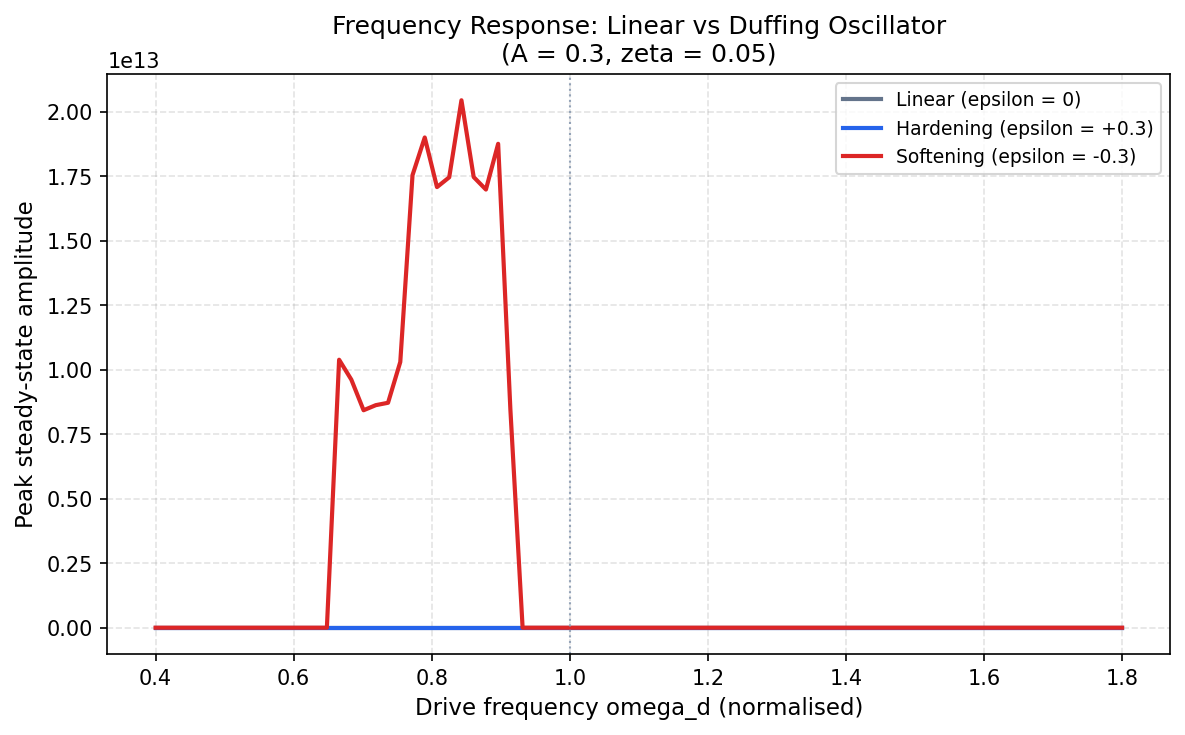

Running the notebook: Copy into a .py file or Jupyter notebook. The bifurcation diagram simulation is the most computationally intensive; expect a few minutes on a standard laptop. Only numpy, scipy, and matplotlib are required.

What to look for: In the frequency response plot, notice how the hardening curve leans right and the softening curve leans left relative to the symmetric linear peak. At higher drive amplitudes (increase A_drive), these curves will develop a fold and you will observe different steady-state values depending on the initial conditions. In the bifurcation diagram, trace the evolution from a single branch (periodic, period-1) through the first split (period-2), subsequent splits, and eventually the dense, continuous scatter of the chaotic regime. The transition between ordered and chaotic regions is not always abrupt; there are windows of periodic behaviour (periodic windows) embedded inside the chaos, another signature of deterministic chaos that random noise would not produce.

References

#

1. Fang, X., Wen, J., Bonello, B., Yin, J., & Yu, D. (2017). Ultra-low and ultra-broad-band nonlinear acoustic metamaterials. Nature Communications, 8, 1288. https://doi.org/10.1038/ncomms11461 (Landmark demonstration of Duffing-resonator acoustic metamaterials with amplitude-dependent and chaotically broadened band gaps; the foundational reference for this post.)

2. Fang, X., Wen, J., Bonello, B., Yin, J., & Yu, D. (2017). Wave propagation in one-dimensional nonlinear acoustic metamaterials. New Journal of Physics, 19, 053007. https://doi.org/10.1088/1367-2630/aa6d49 (Companion theoretical paper; derives wave propagation theory for nonlinear diatomic lattice, showing chaos in the acoustic branch and mechanisms for nonlinear suppression beyond Bragg scattering.)

3. Bae, M. H., & Oh, J. H. (2020). Amplitude-induced bandgap: new type of bandgap for nonlinear elastic metamaterials. Journal of the Mechanics and Physics of Solids, 139, 103930. https://doi.org/10.1016/j.jmps.2020.104066 (Formalises the concept of amplitude-induced band gaps, distinct from linear frequency-based gaps, as a fundamental property class of nonlinear metamaterials.)

4. Sheng, P., Fang, X., Wen, J., & Yu, D. (2021). Vibration properties and optimized design of a nonlinear acoustic metamaterial beam. Journal of Sound and Vibration, 494, 115883. https://doi.org/10.1016/j.jsv.2020.115883 (Systematic parametric study of Duffing-coupled resonator beams; provides design maps linking amplitude, nonlinear stiffness, and chaos onset to attenuation performance.)

5. Fang, X., Wen, J., Benisty, H., & Yu, D. (2020). Ultrabroad acoustical limiting in nonlinear metamaterials due to adaptive-broadening band-gap effect. Physical Review B, 101, 104304. https://doi.org/10.1103/PhysRevB.101.104304 (Distinguishes adaptive band-gap widening from fully chaotic dynamics; demonstrates both mechanisms contribute to ultrabroad suppression and characterises their onset conditions.)

6. Fang, X., Lacarbonara, W., & Cheng, L. (2025). Advances in nonlinear acoustic/elastic metamaterials and metastructures. Nonlinear Dynamics. https://doi.org/10.1007/s11071-024-10219-4 (Comprehensive 2025 review synthesising nonlinear metamaterial design from FPUT chains and granular crystals through to chaos-mediated attenuation; essential current-state reference.)

7. The 2024 acoustic metamaterials roadmap. (2024). Journal of Physics D: Applied Physics, 57, 423001. https://doi.org/10.1088/1361-6463/add306 (Consortium roadmap identifying open problems including the Lyapunov-based design framework gap; positions the research direction pursued in Post 6.)

Series Navigation

#

← Previous: Post 4: Band Gaps and Dispersion - Reading the Map
Next: Post 6: Strange Attractors and Chaos as Design Tool →