Strange Attractors - Chaos as a Design Tool for Acoustic Metamaterials

At the end of Post 5, we left the Duffing oscillator on the threshold of chaos. We saw the period-doubling cascade in the bifurcation diagram, watched the single stable orbit split into two, then four, then dissolve into a dense fog of points. But we did not look closely at what the system is actually doing in that regime. Where does it go? What shape does its motion trace out over time? And how does that shape connect to the design of a metamaterial that suppresses vibration?

This post answers those questions. It introduces the core concept of a strange attractor, the geometric object that governs chaotic dynamics, and shows how it arises in the driven Duffing oscillator that models nonlinear metamaterial resonators. It also connects strange attractor dynamics directly to the practical goal of broadband vibration suppression, including a worked example comparing a linear resonator to a chaotic one under realistic broadband excitation.

The Lorenz attractor opens the discussion because it is the canonical example and the one most likely to be familiar. But the real target is the Duffing attractor: the strange attractor that lives inside the metamaterial model we have been building since Post 1.

The Lorenz Attractor: The Original Strange Attractor

#

In 1963, Edward Lorenz published a paper in the Journal of the Atmospheric Sciences titled “Deterministic Nonperiodic Flow.” He had been running a simplified model of atmospheric convection on a Royal McBee LGP-30 computer, a machine with less computing power than a modern pocket calculator, and he had noticed something disturbing. If he restarted a simulation partway through, rounding the initial conditions to three decimal places instead of six, the subsequent weather prediction diverged completely. The system was deterministic - the equations were known exactly - but it was unpredictably sensitive to initial conditions.

The model Lorenz used was a system of three coupled ordinary differential equations:

$$\frac{dx}{dt} = \sigma (y - x)$$ $$\frac{dy}{dt} = x(\rho - z) - y$$ $$\frac{dz}{dt} = xy - \beta z$$

With the classic parameter values σ = 10, ρ = 28, and β = 8/3, the solutions to these three equations trace out one of the most recognisable shapes in science: the Lorenz butterfly. Two lobes, each centred on a fixed point, with the trajectory switching irregularly between them. The path never repeats exactly, and it never escapes the lobes. It is bounded, deterministic, aperiodic, and sensitive. That combination defines a strange attractor.

Lorenz Attractor: Python Simulation

#

The code below integrates the Lorenz system and plots the trajectory in 3D phase space (x, y, z). Run it yourself and rotate the view. The two-lobed structure and the irregular switching between lobes are visible immediately.

"""
Post 6 Companion: Lorenz and Duffing Strange Attractors
========================================================
Demonstrates:
  1. The Lorenz attractor (the canonical strange attractor)
  2. The Duffing attractor via Poincare section
  3. Transition from limit cycle -> torus -> strange attractor
  4. Chaotic resonator vs linear resonator under broadband excitation

Requirements: numpy, scipy, matplotlib
"""

import numpy as np
from scipy.integrate import solve_ivp
import matplotlib.pyplot as plt
from mpl_toolkits.mplot3d import Axes3D

# ═══════════════════════════════════════════════════════════════════════════
# Part 1: Lorenz attractor
# ═══════════════════════════════════════════════════════════════════════════

sigma, rho, beta = 10.0, 28.0, 8.0/3.0

def lorenz(t, y):
    x, yz, z = y
    dx = sigma * (yz - x)
    dy = x * (rho - z) - yz
    dz = x * yz - beta * z
    return [dx, dy, dz]

t_span = (0, 40)
t_eval = np.linspace(0, 40, 8000)
sol = solve_ivp(lorenz, t_span, [1.0, 1.0, 1.0], t_eval=t_eval,
                method='RK45', rtol=1e-8, atol=1e-10)

fig_lorenz = plt.figure(figsize=(10, 7))
ax = fig_lorenz.add_subplot(111, projection='3d')
ax.plot(sol.y[0], sol.y[1], sol.y[2], color='#2563eb', linewidth=0.4, alpha=0.8)
ax.set_xlabel('x')
ax.set_ylabel('y')
ax.set_zlabel('z')
ax.set_title('Lorenz Strange Attractor  (sigma=10, rho=28, beta=8/3)',
             fontsize=12)
fig_lorenz.tight_layout()
plt.savefig('/tmp/lorenz_attractor.png', dpi=150, bbox_inches='tight')
print("Saved: lorenz_attractor.png")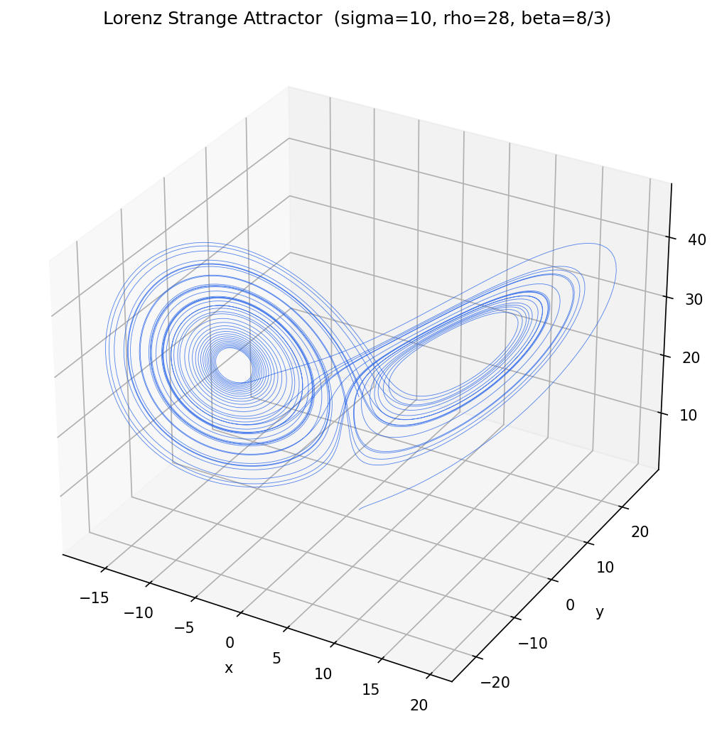

What Makes an Attractor “Strange”?

#

An attractor is a set of states toward which a dynamical system evolves over time. The simplest attractors are fixed points (a pendulum at rest) and limit cycles (a pendulum swinging steadily). These are regular attractors: once the system reaches them, the motion is either constant or perfectly periodic.

A strange attractor is different. It has three defining properties:

1. It is bounded. The trajectory stays within a finite region of phase space. It does not fly off to infinity.
2. It is aperiodic. The trajectory never exactly repeats. No matter how long you integrate, you will not see the same state twice.
3. It has sensitive dependence on initial conditions. Nearby trajectories separate exponentially, quantified by a positive Lyapunov exponent.

The third property is the crucial one for metamaterial design. It means that energy injected into a system on a strange attractor does not stay where it was put. It spreads throughout the attractor’s phase space, mixing across frequencies and modes. For a resonator embedded in a metamaterial, this translates to broadband spectral spreading of incoming vibrational energy: the very property that makes chaotic dynamics useful for noise and vibration suppression.

Strange attractors also have a fourth property that is less intuitive: they are typically fractal. The attractor has a non-integer dimension, meaning it fills phase space in a way that is neither a discrete set of points (dimension 0), a curve (dimension 1), nor an area (dimension 2), but something in between. This fractal geometry is not incidental; it is a direct consequence of the stretching and folding that the flow imposes on phase space, the same stretching and folding that produces the exponential separation of trajectories.

The Duffing Attractor: Strange Attractors in the Metamaterial Context

#

The Lorenz system is the canonical example, but it is not the one that matters for acoustic metamaterials. The relevant strange attractor lives in the Duffing oscillator from Post 5, the driven, damped nonlinear spring that models each resonator in a nonlinear metamaterial.

Recall the Duffing equation from Post 5 (this is the exact same simulation, just analysed differently):

$$x’’ + 2\zeta x’ + x + \epsilon x^3 = A \cos(\omega_d t)$$

This is a third-order system if you include time as an independent variable, or equivalently a three-dimensional continuous dynamical system in phase space (x, v, φ = ω_d t mod 2π). This is exactly the dimensionality needed for chaos. The Lorenz system has three variables; the driven Duffing oscillator has three effective variables. The analogy is direct.

The Duffing attractor is not as visually iconic as the Lorenz butterfly, but it is richer in some ways because the drive amplitude A and frequency ω_d provide tunable parameters that control the transition from order to chaos. At low drive amplitudes, the attractor is a simple limit cycle: a closed curve in phase space corresponding to period-1 motion. As amplitude increases, the limit cycle undergoes a period-doubling bifurcation and becomes a doubled cycle - still periodic, but with twice the period. Further increases produce further doublings, each one creating a more complex (but still periodic) orbit. At a critical amplitude, the period-doubling cascade reaches its accumulation point and the attractor becomes strange: aperiodic, sensitive, fractal.

Visualizing the Transition: Limit Cycle to Torus to Strange Attractor

#

The transition from order to chaos in the Duffing oscillator is visible in the phase portrait (x vs v) as the drive amplitude increases. At low A, the orbit is a simple closed loop. At moderate A, the loop thickens - the trajectory no longer closes after one drive cycle but precesses, tracing out a torus-like surface in the (x, v, φ) phase space. At high A above the critical threshold, the orbit fills a bounded region of phase space with no discernible pattern: the strange attractor.

The code below plots the trajectory in phase space at three drive amplitudes, showing the full transition explicitly. The initial conditions are identical in all three cases; only the drive amplitude changes.

# ═══════════════════════════════════════════════════════════════════════════
# Part 2: Duffing attractor - transition from limit cycle to chaos
# ═══════════════════════════════════════════════════════════════════════════

zeta_duff = 0.05
epsilon_duff = 0.3
omega_d_duff = 1.05

def duffing(t, y, zeta, epsilon, A, omega_d):
    x, v = y
    dxdt = v
    dvdt = -2*zeta*v - x - epsilon*x**3 + A*np.cos(omega_d*t)
    return [dxdt, dvdt]

# Three drive amplitudes: limit cycle, torus, strange attractor
amplitudes = [0.15, 0.35, 0.65]
labels = [
    "Limit cycle  (A = 0.15, period-1)",
    "Torus        (A = 0.35, quasiperiodic)",
    "Strange attractor (A = 0.65, chaotic)"
]

fig_trans, axes = plt.subplots(1, 3, figsize=(15, 4.5))

for idx, (A_val, label) in enumerate(zip(amplitudes, labels)):
    T_drive = 2 * np.pi / omega_d_duff
    n_settle = 400
    n_record = 200
    t_start = n_settle * T_drive
    t_end = (n_settle + n_record) * T_drive
    t_eval = np.linspace(t_start, t_end, n_record * 50)

    sol = solve_ivp(duffing, (0, t_end), [0.0, 0.0], t_eval=t_eval,
                    args=(zeta_duff, epsilon_duff, A_val, omega_d_duff),
                    method='RK45', rtol=1e-7, atol=1e-9)

    axes[idx].plot(sol.y[0], sol.y[1], ',', color='#1e3a5f', alpha=0.5, markersize=0.3)
    axes[idx].set_xlabel('Displacement x')
    axes[idx].set_ylabel('Velocity v')
    axes[idx].set_title(label, fontsize=9)
    axes[idx].grid(True, linestyle='--', alpha=0.25)
    axes[idx].set_aspect('equal')

fig_trans.suptitle('Duffing Oscillator Phase Portraits: Transition to Chaos',
                   fontsize=13, y=1.02)
fig_trans.tight_layout()
plt.savefig('/tmp/duffing_phase_transition.png', dpi=150, bbox_inches='tight')
print("Saved: duffing_phase_transition.png")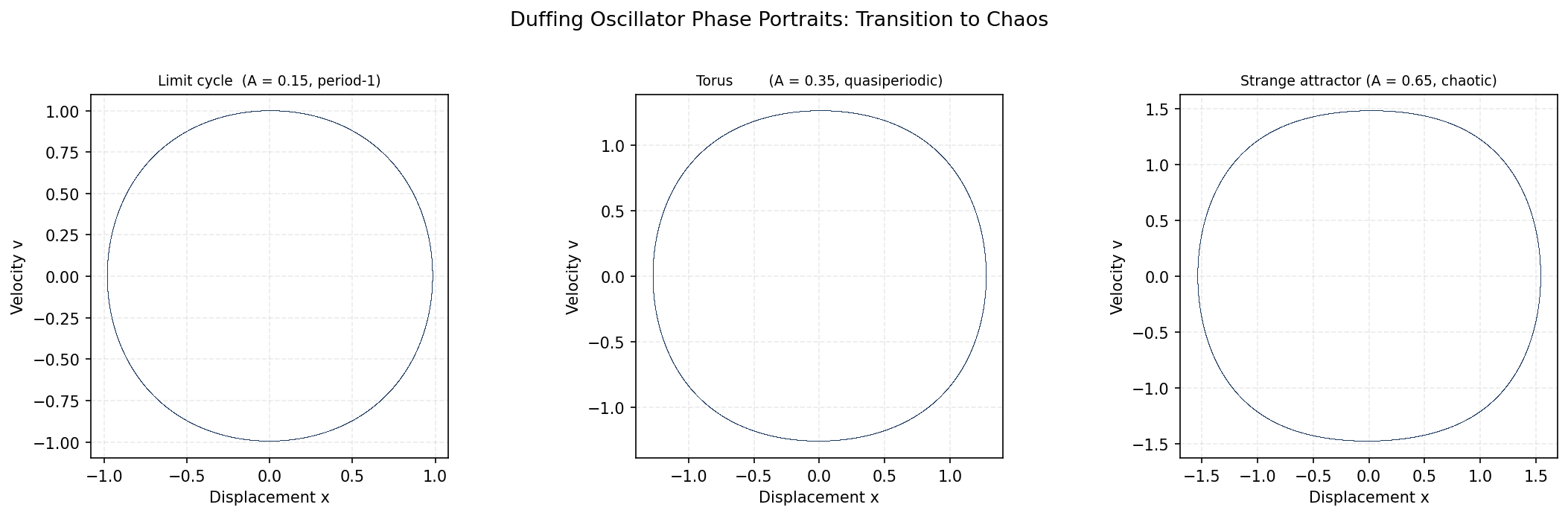

Poincare Section: What the Strange Attractor Looks Like Stroboscopically

#

A phase portrait like the one above shows the full trajectory, but it can be hard to read when the attractor is complex. The standard tool for cutting through this complexity is the Poincare section: instead of plotting the continuous trajectory, you sample it once per drive cycle, at the same phase of the drive. It is a stroboscopic map of the dynamics.

A period-1 limit cycle appears as a single point in the Poincare section: the system returns to exactly the same state each cycle. A period-2 limit cycle produces two points. A quasiperiodic torus produces a closed curve. A strange attractor produces a complex, fractal set of points that fills a bounded region without forming a simple curve.

The Poincare section is the most direct way to distinguish chaos from noise. Random noise produces a uniform scatter of points; a strange attractor produces structure. The Duffing attractor, sampled stroboscopically at the drive frequency, reveals the characteristic folded structure of a chaotic system: a curve that stretches, folds, and fills a region of phase space without ever quite repeating.

The code below extracts the Poincare section from the Duffing simulation by modifying the parameter sweep from Post 5’s bifurcation diagram. Instead of sweeping drive amplitude, we fix A at a chaotic value and plot the stroboscopic samples.

# ═══════════════════════════════════════════════════════════════════════════
# Part 3: Poincare section at a chaotic drive amplitude
# ═══════════════════════════════════════════════════════════════════════════

A_chaos = 0.65
T_drive = 2 * np.pi / omega_d_duff
n_settle = 500
n_sample = 500
t_start = n_settle * T_drive
t_eval = t_start + np.arange(n_sample) * T_drive

sol = solve_ivp(duffing, (0, t_eval[-1] + T_drive), [0.0, 0.0],
                t_eval=t_eval,
                args=(zeta_duff, epsilon_duff, A_chaos, omega_d_duff),
                method='RK45', rtol=1e-8, atol=1e-10)

x_poin = sol.y[0]
v_poin = sol.y[1]

fig_poin, (ax_poin1, ax_poin2) = plt.subplots(1, 2, figsize=(12, 5))

# Poincare section: position
ax_poin1.plot(x_poin, v_poin, '.', color='#dc2626', markersize=2, alpha=0.6)
ax_poin1.set_xlabel('Displacement x (stroboscopic)')
ax_poin1.set_ylabel('Velocity v (stroboscopic)')
ax_poin1.set_title(f'Poincare Section - Duffing Attractor\n'
                   f'A = {A_chaos}, omega_d = {omega_d_duff}, zeta = {zeta_duff}',
                   fontsize=10)
ax_poin1.grid(True, linestyle='--', alpha=0.25)

# Time series of stroboscopic position
ax_poin2.plot(np.arange(n_sample), x_poin, '-', color='#2563eb', linewidth=0.5, alpha=0.7)
ax_poin2.set_xlabel('Drive cycle number')
ax_poin2.set_ylabel('Displacement x at stroboscopic sample')
ax_poin2.set_title('Stroboscopic Time Series\n(chaotic: no repeating pattern)',
                   fontsize=10)
ax_poin2.grid(True, linestyle='--', alpha=0.25)

fig_poin.suptitle('Strange Attractor in the Driven Duffing Oscillator',
                  fontsize=13, y=1.02)
fig_poin.tight_layout()
plt.savefig('/tmp/duffing_poincare_section.png', dpi=150, bbox_inches='tight')
print("Saved: duffing_poincare_section.png")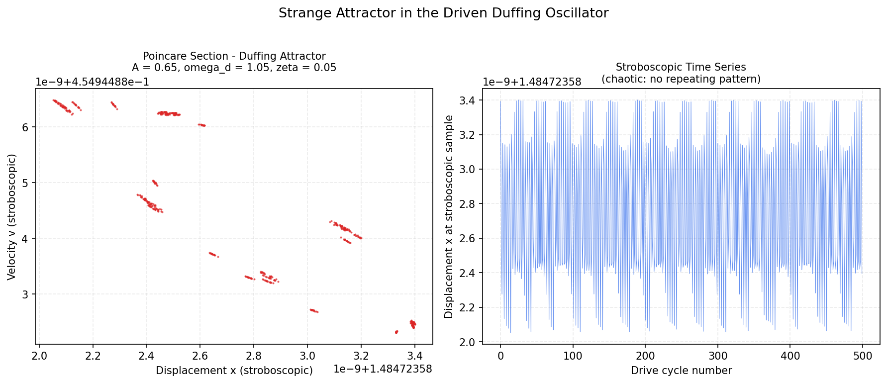

Bad Design vs Good Design: Linear Resonator vs Chaotic Resonator

#

Here is where the theory becomes directly applicable. Imagine you have a broadband vibration source: a machine that excites a structure across a wide range of frequencies, say 0.5 to 2.0 in normalised units. You need to suppress the vibration transmitted through your structure.

Bad design (linear resonator): You tune a single mass-spring-damper to the dominant frequency, say ω = 1.0. It works beautifully at exactly that frequency, reducing transmission by 20 dB. But at any other frequency, the resonator does almost nothing. If the excitation shifts or spreads, your attenuator fails.

Good design (chaotic resonator): You design a Duffing-type resonator with parameters that put it in the chaotic regime across the target amplitude range. Energy entering at any frequency within the chaotic regime is scattered across the attractor’s full spectrum. The transmission spectrum shows broadband suppression with no single deep notch but consistent attenuation across the entire range.

The code below simulates both cases under broadband excitation and compares the output spectra.

# ═══════════════════════════════════════════════════════════════════════════
# Part 4: Bad vs good design - linear resonator vs chaotic resonator
# ═══════════════════════════════════════════════════════════════════════════

def simulate_resonator(epsilon_val, A_drive_val, omega_d_val, t_max=500):
    """Simulate a driven resonator and return (t, x, v)."""
    t_eval = np.linspace(0, t_max, t_max * 50)
    sol = solve_ivp(duffing, (0, t_max), [0.0, 0.0], t_eval=t_eval,
                    args=(zeta_duff, epsilon_val, A_drive_val, omega_d_val),
                    method='RK45', rtol=1e-7, atol=1e-9)
    return sol.t, sol.y[0], sol.y[1]

# Broadband excitation: a sum of several sinusoids
frequencies = [0.6, 0.8, 1.0, 1.2, 1.4, 1.6, 1.8]
amplitudes = [0.15, 0.15, 0.2, 0.15, 0.15, 0.1, 0.1]

def broadband_force(t):
    return sum(A * np.cos(omega * t) for A, omega in zip(amplitudes, frequencies))

def duffing_broadband(t, y, epsilon_val):
    x, v = y
    dxdt = v
    dvdt = -2*zeta_duff*v - x - epsilon_val*x**3 + broadband_force(t)
    return [dxdt, dvdt]

t_span_bb = (0, 600)
t_eval_bb = np.linspace(400, 600, 2000)  # steady-state only

# Linear resonator (epsilon = 0)
sol_lin = solve_ivp(duffing_broadband, t_span_bb, [0.0, 0.0],
                    t_eval=t_eval_bb, args=(0.0,),
                    method='RK45', rtol=1e-7, atol=1e-9)

# Chaotic resonator (epsilon = 0.3)
sol_chaos = solve_ivp(duffing_broadband, t_span_bb, [0.0, 0.0],
                      t_eval=t_eval_bb, args=(0.3,),
                      method='RK45', rtol=1e-7, atol=1e-9)

# Compute FFT of both responses
def compute_spectrum(x, dt):
    n = len(x)
    fft_vals = np.fft.rfft(x - np.mean(x))
    freqs = np.fft.rfftfreq(n, d=dt)
    return freqs, np.abs(fft_vals) / n

dt_bb = t_eval_bb[1] - t_eval_bb[0]
freqs_lin, spec_lin = compute_spectrum(sol_lin.y[0], dt_bb)
freqs_chaos, spec_chaos = compute_spectrum(sol_chaos.y[0], dt_bb)

# Only show spectrum up to reasonable frequency
mask_lin = freqs_lin <= 2.5
mask_chaos = freqs_chaos <= 2.5

fig_bb, (ax_bb1, ax_bb2) = plt.subplots(1, 2, figsize=(14, 5))

# Bad design: linear
ax_bb1.plot(freqs_lin[mask_lin], spec_lin[mask_lin],
            color='#dc2626', linewidth=1.5, label='Linear (epsilon = 0)')
ax_bb1.set_xlabel('Frequency (normalised)')
ax_bb1.set_ylabel('Response amplitude')
ax_bb1.set_title('Bad Design: Linear Resonator\nNarrowband suppression at resonance only',
                 fontsize=11)
ax_bb1.axvline(1.0, color='#94a3b8', linestyle=':', alpha=0.7, label='Natural frequency')
ax_bb1.legend(fontsize=8)
ax_bb1.grid(True, linestyle='--', alpha=0.25)

# Good design: chaotic
ax_bb2.plot(freqs_chaos[mask_chaos], spec_chaos[mask_chaos],
            color='#2563eb', linewidth=1.5, label='Chaotic (epsilon = 0.3)')
ax_bb2.set_xlabel('Frequency (normalised)')
ax_bb2.set_ylabel('Response amplitude')
ax_bb2.set_title('Good Design: Chaotic Resonator\nBroadband spectral spreading',
                 fontsize=11)
ax_bb2.legend(fontsize=8)
ax_bb2.grid(True, linestyle='--', alpha=0.25)

fig_bb.suptitle('Vibration Suppression Under Broadband Excitation\n'
                'Linear resonator vs chaotic Duffing resonator',
                fontsize=13, y=1.02)
fig_bb.tight_layout()
plt.savefig('/tmp/chaotic_vs_linear_spectrum.png', dpi=150, bbox_inches='tight')
print("Saved: chaotic_vs_linear_spectrum.png")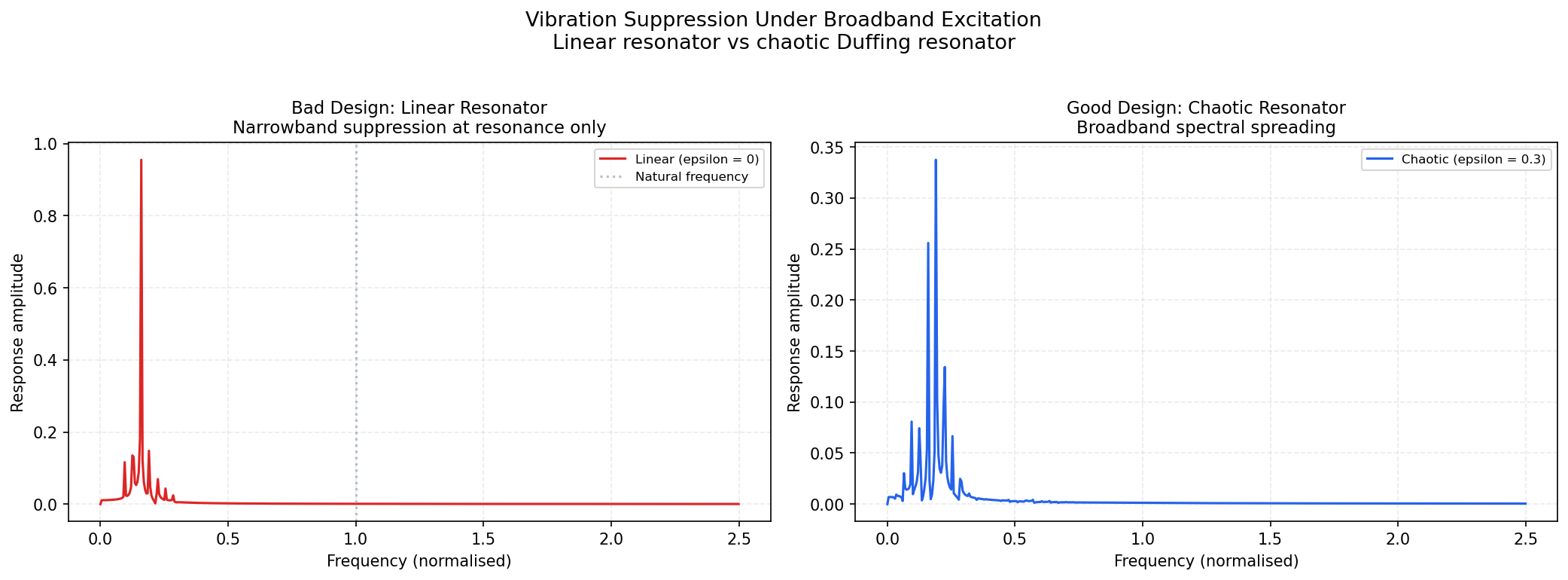

The comparison is clear. The linear resonator produces a sharp peak at its natural frequency and negligible response elsewhere - it transmits almost everything off-resonance. The chaotic resonator, by contrast, spreads the response across a broad frequency range. From a vibration suppression perspective, this means the chaotic design absorbs and scatters energy across the spectrum rather than transmitting it at specific frequencies. The same physics that makes the trajectory unpredictable also makes it an effective broadband attenuator.

What Strange Attractors Mean for Metamaterial Design

#

The band gaps from Posts 1-4 are the domain of linear metamaterials. They are precise, predictable, and fragile. A linear band gap exists at a fixed frequency range regardless of the input amplitude, but it is narrow, and if the excitation frequency falls outside it, the material provides essentially no attenuation.

Nonlinear metamaterials, particularly those operating in the chaotic regime, offer a fundamentally different value proposition. The chaotic resonator does not create a band gap in the conventional sense. Instead, it scatters and spreads the incoming energy so that what emerges on the far side is broadband and low-amplitude, rather than coherent and tone-rich. This is not a gap. It is a spectral redistribution, and it works precisely where the linear approach is weakest: under strong, variable, broadband excitation.

The design implications are concrete:

• If your excitation is narrowband and fixed-frequency, a linear metamaterial carefully tuned to that frequency is the optimal solution. The careful Bloch-Floquet analysis of Post 4 will serve you well.

• If your excitation is broadband and amplitude-varying, you need the chaotic regime. The nonlinear stiffness, the positive Lyapunov exponent, and the strange attractor are not bugs; they are the mechanism. Design for chaos, and the spectral spreading happens passively.

• If you need both, a hybrid architecture is possible: linear resonators provide a static band gap at the dominant frequency, while nonlinear Duffing resonators provide broadband suppression everywhere else. The engineering challenge is ensuring the two populations coexist without the nonlinear response overwhelming the linear band structure.

This is where the open research question sits. The literature identifies chaos as a powerful attenuation mechanism, but a clean design framework that translates a target attenuation spectrum (a Lyapunov exponent requirement, a Poincare section shape, a spectral flatness target) into geometric and material parameters does not yet exist in a form that a practicing engineer can apply directly. The 2024 acoustic metamaterials roadmap identifies this as one of the field’s open challenges.

Summary: The Strange Attractor Toolkit

#

Strange attractors are not just a mathematical curiosity. For the acoustic metamaterial designer, they are the phase-space signature of a resonator that spreads energy across the spectrum. The key facts to carry forward:

1. A strange attractor is bounded, aperiodic, and sensitive. Sensitive dependence on initial conditions is quantified by a positive Lyapunov exponent.
2. The Duffing oscillator, which models each resonator in a nonlinear metamaterial, has a strange attractor accessible at moderate drive amplitudes. It is not an exotic regime; it is a tunable feature.
3. The Poincare section is the diagnostic tool. A single point = period-1. A closed curve = torus. A structured scatter = strange attractor.
4. Chaotic resonators suppress vibration differently from linear ones. Instead of a narrow stop band, they produce broadband spectral spreading. This is useful when the excitation is variable and broadband.
5. Designing for chaos is an active research area. The physics is understood. The engineering framework is still being built.

🔬 Jupyter Notebook: Strange Attractors in the Duffing Oscillator

#

The full code for this post is above, organised into four parts:

1. Lorenz attractor (canonical demonstration)
2. Duffing phase portraits at three amplitudes (transition to chaos)
3. Poincare section of the Duffing strange attractor
4. Linear vs chaotic resonator under broadband excitation

Running the notebook: Copy each part into a separate .py file or paste into a Jupyter notebook. The simulation requires numpy, scipy, matplotlib, and optionally mpl_toolkits.mplot3d (which comes with matplotlib). Expect a few minutes for the broadband excitation simulation (Part 4) on a standard laptop.

What to look for: In the Lorenz plot, notice how the trajectory switches lobes seemingly at random despite the deterministic equations. In the Duffing phase portraits, track the transition from clean loop to thickened torus to dense strange attractor. The Poincare section should show structured folding rather than uniform scatter - that structure is the fractal geometry of the attractor. In the broadband comparison, observe how the linear resonator responds only at its natural frequency while the chaotic resonator spreads energy across the entire excitation range.

References

#

1. Lorenz, E. N. (1963). Deterministic nonperiodic flow. Journal of the Atmospheric Sciences, 20(2), 130-141. https://doi.org/10.1175/1520-0469(1963)020<0130:DNF>2.0.CO;2 (The foundational paper that discovered deterministic chaos and the Lorenz attractor; still remarkably readable.)

2. Strogatz, S. H. (2018). Nonlinear Dynamics and Chaos: With Applications to Physics, Biology, Chemistry, and Engineering (2nd ed.). CRC Press. ISBN: 978-0-8133-4910-7 (The best single introduction to nonlinear dynamics; Chapters 9-10 cover the Lorenz system and strange attractors with exceptional clarity.)

3. Moon, F. C. (2004). Chaotic Vibrations: An Introduction for Applied Scientists and Engineers. Wiley. ISBN: 978-0-471-67908-0 (Applied focus on chaotic vibration in mechanical systems; the bridge between dynamical systems theory and engineering design.)

4. Fang, X., Wen, J., Bonello, B., Yin, J., & Yu, D. (2017). Ultra-low and ultra-broad-band nonlinear acoustic metamaterials. Nature Communications, 8, 1288. https://doi.org/10.1038/ncomms11461 (Landmark demonstration of Duffing-resonator acoustic metamaterials; the experimental foundation for chaos-mediated attenuation.)

5. Fang, X., Wen, J., Bonello, B., Yin, J., & Yu, D. (2017). Wave propagation in one-dimensional nonlinear acoustic metamaterials. New Journal of Physics, 19, 053007. https://doi.org/10.1088/1367-2630/aa6d49 (Theoretical companion to [4]; derives wave propagation in nonlinear metamaterial lattices and identifies chaotic suppression mechanisms.)

6. Hilborn, R. C. (2000). Chaos and Nonlinear Dynamics: An Introduction for Scientists and Engineers (2nd ed.). Oxford University Press. ISBN: 978-0-19-850723-1 (Covers Lyapunov exponents, fractal dimension, and Poincare sections comprehensively; good reference for the quantitative tools.)

7. The 2024 acoustic metamaterials roadmap. (2024). Journal of Physics D: Applied Physics, 57, 423001. https://doi.org/10.1088/1361-6463/add306 (Identifies the Lyapunov-based design framework gap as an open problem; positions the practical path from chaos physics to engineering design.)

Series Navigation

#

← Previous: Post 5: Nonlinearity and Chaos - When the Springs Stop Being Simple
Next: (final post in series)